
Synthetic DID and its implementation in Stata
Published:
As one can tell from the name, synthetic DID is a combination of synthetic control and DID. One main challenge of DID is the validation of parallel trend assumption, as it not always holds in the data that treated and control groups have identical trend or characteristics prior to the treatment event. Built on the method of synthetic control, synthetic DID loosens the needs for parallel assumption by constructing matched control units.
In this post, I will cover
Synthetic DID
In this section, I first present a comparison between synthetic control, DID, synthetic DID, and discuss the prerequisites for the application of synthetic DID. Then the main focus is the methodology of synthetic DID, including how to find the optimal unit-specific and time-specific weights, how to estimate the variance of the treatment effect. Finally, two extensions, incorporating covariates and staggered adoption, are introduced.
Comparison of synthetic control, DID and synthetic DID
The table below shows a comparison between synthetic control, DID and synthetic DID.
| Unit-specific weight | Time-specific weight | Fixed effect | |
|---|---|---|---|
| Synthetic control | ✓ | ✖️ | Time FE |
| DID | ✖️ | ✖️ | Time FE and unit FE |
| Synthetic DID | ✓ | ✓ | Time FE and unit FE |
Requirements of synthetic DID
The following requirements must be satisfied before performing synthetic DID.
- Balanced panel data (N units, T periods) without missing or gap
- Once treated, units are assumed to remain treated forever
- No always treated units
- At least two pre-treatment periods
Synthetic DID methodology
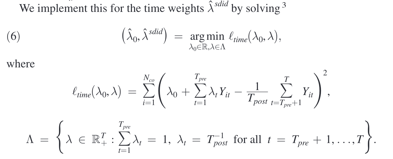
The goal of synthetic DID is to estimate the average treatment effect in absence of perfectly matched control units in original data. Similar to synthetic control approach, it selects optimal unit-specific weight to minimize the absolute difference between the treated unit and the synthetic control units over all pre-treatment period, allowing for a constant level difference. Further, it selects optimal time-specific weight (for pre-treatment period) to minimize the absolute difference between the pre-treatment and post-treatment control units.
Specifically, the optimization problems are formed as follows (Arkhangelsky et al., 2021). 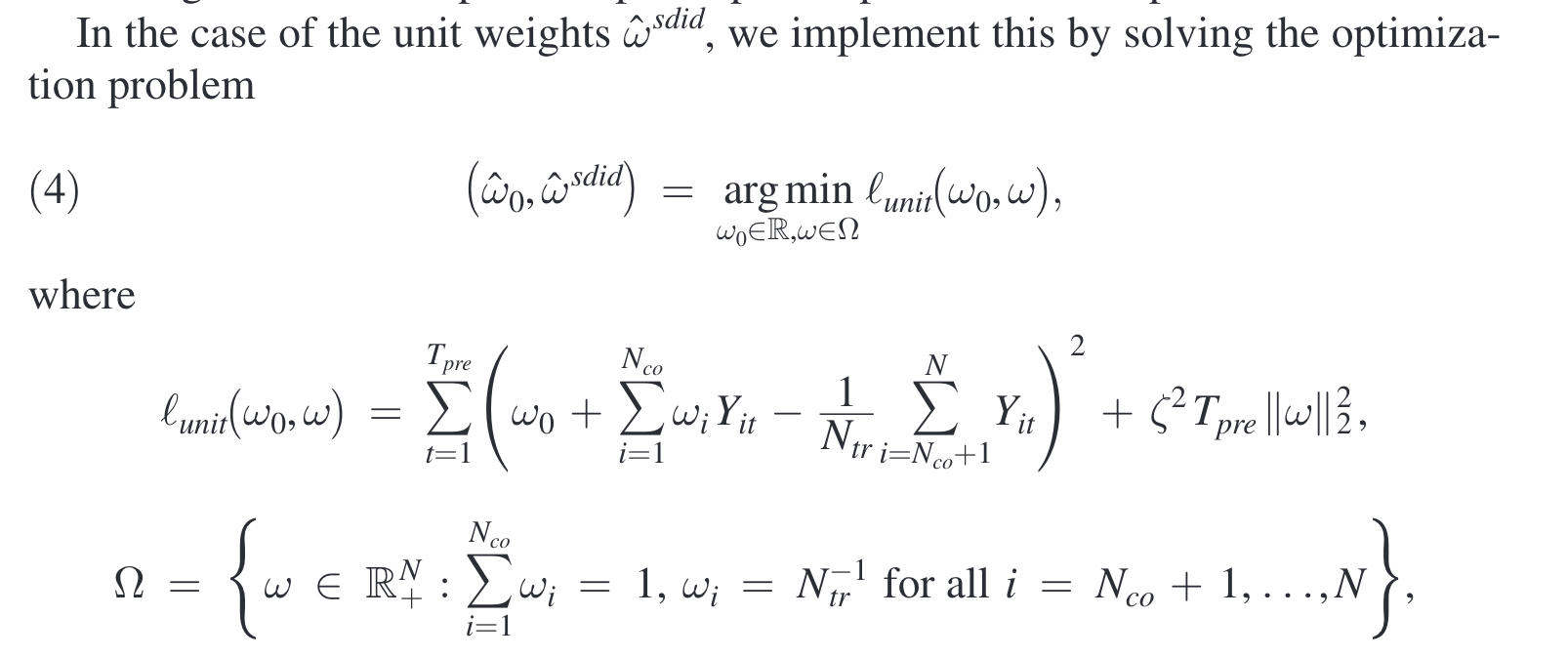
There are three approaches to estimate the variance of the treatment effect $\hat{\tau}^{sdid}$. Without going into the details, I summarize each approach and their pros and cons.
- Bootstrap: resample and re-estimate $\hat{\tau}^{sdid}$ to compute the variance. It is observed in simulation to have particularly good properties, but it is computationally expensive with large samples or where covariates are included, and it may be unreliable when the number of treated units is small (the proof of asymptotic normality rely on the number of treated units being large).
- Jackknife: iterate over all units in the data, in each iteration remove the given unit, and recalculate $\hat{\tau}^{sdid}$ using the optimal unit-specific and time-specific weights estimated in original specification. It saves the computational power of re-estimating optimal weights, but it is not applicable when there is only one treated unit in each treatment period. Same as for bootstrap, it may be unreliable when the number of treated units is small.
- Placebo: conserve only the control units, then randomly assign the same treatment structure to these control units as a placebo treatment, re-estimate $\hat{\tau}^{sdid}$, repeat the procedure to compute the variance. It overcomes the limit when the number of treated units is small, but requires homoskedasticity across units.
Extensions
With covariates As a pre-processing step, regress the outcome variable on covariates, and use the residuals for synthetic DID. It removes the impact of changes in covariates from the outcome before calculating the synthetic control. Note that the role of covariates in synthetic DID is different from its role in synthetic control, where the treated and synthetic control units are matched based on covariates.
Staggered adoption The whole sample with staggered adoption can be broken down into adoption date specific subsamples. Each subsample includes the treated units with the same adoption date, and all control units which are never treated. The average treatment effect can then be calculated by applying the synthetic DID estimator to each of these adoption-specific subsamples, and calculating a weighted average of these estimators, where weights are assigned based on the relative number of post-treatment periods of treated units in each adoption group.
Stata Implementation
To implement synthetic DID in Stata, we could use sdid package by Daniel Pailañir and Damian Clarke. It can be installed easily with ssc install sdid.
In the rest of the post, I explain its basic syntax and provide a simple example with one-time treatment. More details on the Stata package can be found on github or in Damian Clarke et al. (2023).
Basic Syntax
The command syntax is as follows.
sdid depvar groupvar timevar treatment [if] [in], vce(type)
[covariates(varlist, type) seed(#) reps(#) method(type)
graph g1on g1_opt(string) g2_opt(string) graph_export(string, type)
msize(markersizestyle) unstandardized mattitles]
- depvar: dependent variable
- groupvar: unit (entity) id
- timevar: time periods
- treatment: treat*post dummy
- vce(type): choose from following approaches
- bootstrap: greater than one unit is treated
- jackknife: greater than one unit is treated in each treatment period (if multiple treatment periods are considered)
- placebo: at least one more control than treated unit
- noinference: only generate point estimates
- covariates(varlist, type): varlist specifies the covariates used to adjust treatment and control units, type includes following approaches
- optimized: follow Arkhangelsky et al. (2021)
- projected: follow Kranz (2022), more stable and faster in some cases
- seed(#): seed for pseudo-random numbers
- reps(#): the number of repetitions used in the calculation of bootstrap and placebo standard errors, default 50 iterations
- method(type):
- sdid: default, synthetic DID
- sc: synthetic control
- did: DID
- g1on: include unit-specific weight graph, default off
- g1_opt: option for unit-specific weight graph, consistent with twoway scatter plots
- g2_opt: option for outcome trend graph, consistent with twoway line plots
- graph_export(string, type): string specifies the prefix of graph name, type specifies graph type, i.e., “.eps”, “.pdf”
- msize(markersizestyle): modify the size of marker in graph 1
- unstandardized: if controls are included, the optimized method and unstandardized option is specified, controls will be entered in their original units, default standardized as Z-scores
- mattitles: requests labels to be added to the returned e(omega) weight matrix providing names (in string) for the unit variables which generate the synthetic control group in each case
Replication of Arkhangelsky et al. (2021)
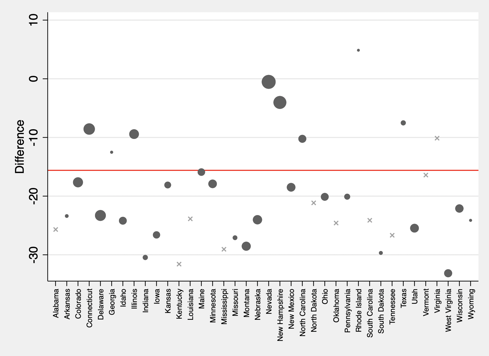
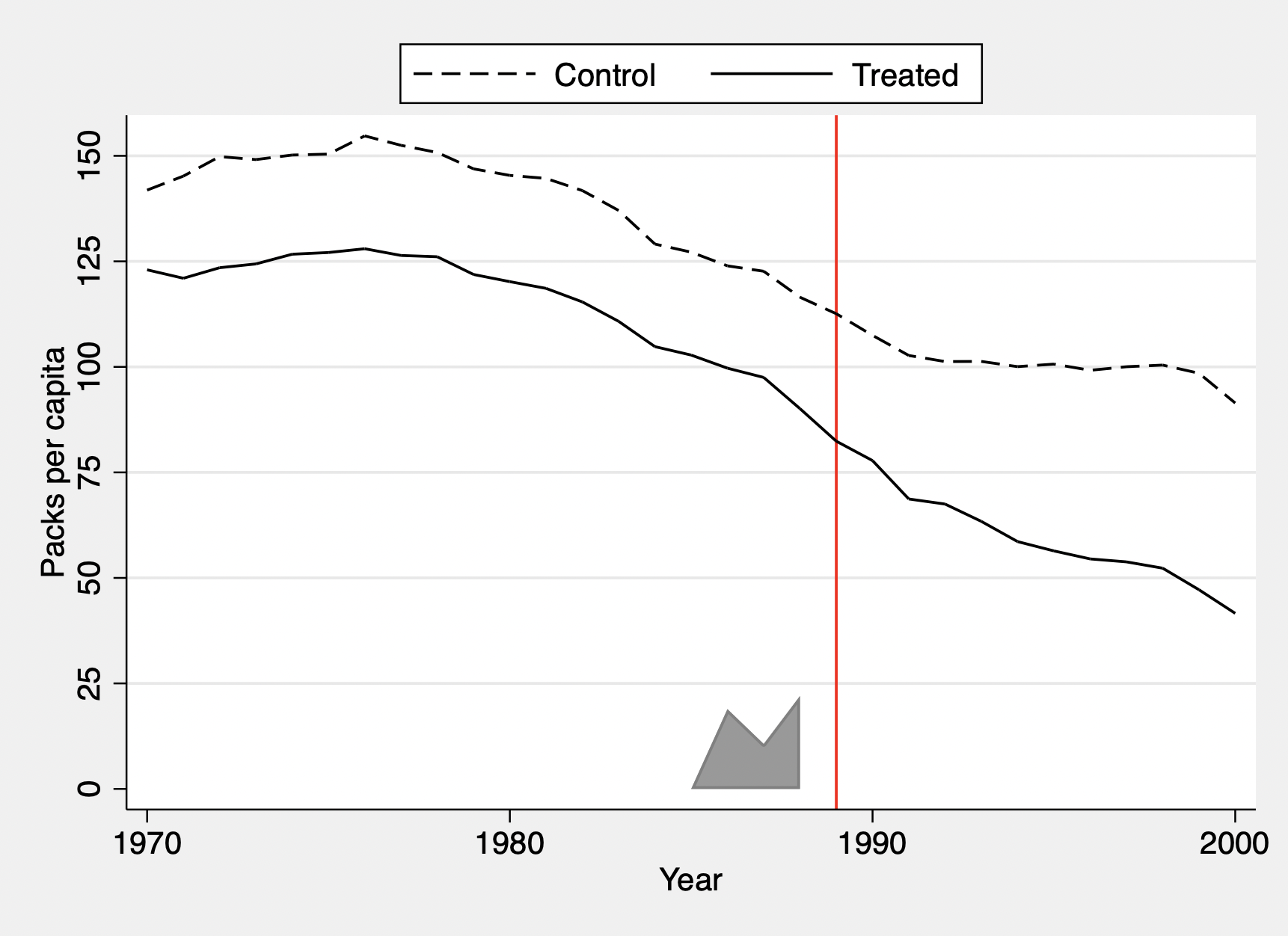
The commands below estimate the treatment effect and plot the time trend for treated and synthetic control unit.
sdid packspercapita state year treated, vce(placebo) seed(1213)
graph g2_opt(ylabel(0(25)150) ytitle("Packs per capita") scheme(sj))
g1_opt(xtitle("") scheme(sj)) g1on graph_export(sdid_, .eps)

Placebo replications (50). This may take some time.
----+--- 1 ---+--- 2 ---+--- 3 ---+--- 4 ---+--- 5
..................................................     50


Synthetic Difference-in-Differences Estimator

-----------------------------------------------------------------------------
packsperca~a |     ATT     Std. Err.     t      P>|t|    [95% Conf. Interval]
-------------+---------------------------------------------------------------
     treated | -15.60383    9.00803    -1.73    0.083   -33.25924     2.05158
-----------------------------------------------------------------------------
95% CIs and p-values are based on Large-Sample approximations.
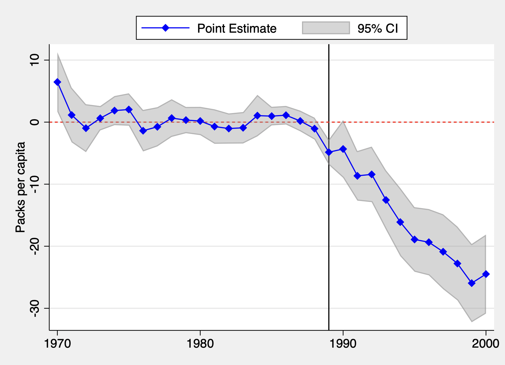
The commands below create the event study plot of the difference between treated and control units and the associated confidence interval.
// n = number of pre-treatment periods
// T = number of periods
local n = 19
local T = 31
qui sdid packspercapita state year treated, vce(noinference) graph
// save lambda weight (pre-treatment periods)
matrix lambda = e(lambda)[1..`n',1]
// control baseline (pre-treatment periods)
matrix yco = e(series)[1..`n',2]
// treated baseline (pre-treatment periods)
matrix ytr = e(series)[1..`n',3]
// calculate the pre-treatment mean	(meanpre_o)
matrix aux = lambda'*(ytr - yco)
scalar meanpre_o = aux[1,1]

// store Ytr-Yco (both pre and post periods)
matrix difference = e(difference)[1..`T',1..2]
svmat difference
ren (difference1 difference2) (time d)
// calculate differences between treated units and synthetic controls post treatment compared to pre treatment
replace d = d - meanpre_o

// bootstrap process
local b = 1
local B = 50
while `b'<=`B' {
	preserve
	bsample, cluster(state) idcluster(c2)
	qui count if treated == 0
	local r1 = r(N)
	qui count if treated != 0
	local r2 = r(N)
	if (`r1'!=0 & `r2'!=0) {
		qui sdid packspercapita c2 year treated, vce(noinference) graph
		matrix lambda_b = e(lambda)[1..`n',1]
		matrix yco_b = e(series)[1..`n',2]
		matrix ytr_b = e(series)[1..`n',3]
		matrix aux_b = lambda_b'*(ytr_b - yco_b)
		matrix meanpre_b = J(`T',1,aux_b[1,1])
		matrix d`b' = e(difference)[1..`T',2] - meanpre_b
		local ++b
	}
restore
}

// calculate standard deviation
preserve
keep time d
keep if time!=.
// import each bootstrap replicate of difference between trends
forval b=1/`B' {
	svmat d`b'
}
// calculate standard deviation of this difference
egen rsd = rowsd(d11 - d`B'1)
// lower bounds on bootstrap CIs
gen LCI = d + invnormal(0.025)*rsd
// upper bounds on bootstrap CIs
gen UCI = d + invnormal(0.975)*rsd

// generate plot
tw rarea UCI LCI time, color(gray%40) || connected d time, color(blue) m(d) xtitle("")
ytitle("Packs per capita") legend(order(2 "Point Estimate" 1 "95% CI") pos(12) col(2))
xline(1989, lc(grey) lp(solid)) yline(0, lc(red) lp(shortdash)) scheme(sj)
graph export "event_study.pdf", replace
restore
There are also R packages available for the implementation of synthetic DID.
Reference
- Abadie, Alberto, Alexis Diamond, and Jens Hainmueller,2010, Synthetic Control Methods for Comparative Case Studies: Estimating the Effect of California’s Tobacco Control Program. Journal of the American Statistical Association 105 (490): 493–505.
- Arkhangelsky, Dmitry, Susan Athey, David A. Hirshberg, Guido W. Imbens, and Stefan Wager, 2021, Synthetic Difference-in-Differences. American Economic Review 111 (12): 4088–4118.
- Damian Clarke, Daniel Pailañir, Susan Athey, and Guido Imbens, 2023, Synthetic Difference-in-Differences Estimation. IZA Discussion Paper.
- Daniel Pailañir and Damian Clarke, sdid–Synthetic Difference-in-Differences for Stata. Stata package.
- Kranz Sebastian, 2021, Synthetic Difference-in-Differences with Time Varying Covariates. Technical report.