“Difference-in-Differences When Parallel Trends Might Be Violated” by Jonathan Roth

The Validity of difference-in-differences relies on the parallel trends (PT) assumption. Namely, in the absence of the treatment, the treatment and control groups would have followed a similar trend over time. This assumption allows us to attribute any difference in outcomes after the treatment to the treatment itself, rather than other confounding factors.

However, we are often unsure about the validity of this assumption ex-ante. Why?

• Treatment status may be correlated with time-varying confounds.
• Parallel trend is often sensitive to the choice of functional form, as it can hold in levels but not logs and vice versa (Roth and Sant’Anna, 2021).

In existing DiD studies, researchers plot the pre-treatment effect as a plausibility test (pre-trends test), to show we cannot reject the null hypothesis that the pre-treatment effect is significant from zero. However, it is important to be aware of its limitations.

What are the limitations of pre-trends testing?

1. Low power

One limitation of pre-trends testing is low power, which refers to the inability to detect significant pre-trend even if PT is violated. This often arises due to the noisy data.

Here is an example using He and Wang (2017).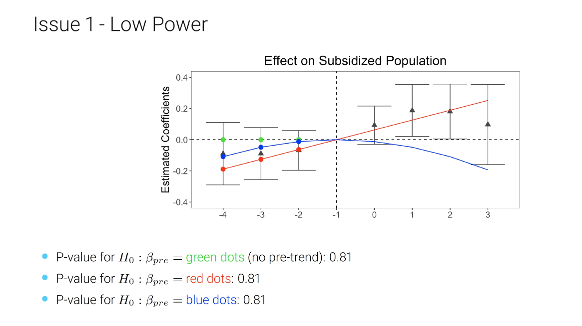

It is true that we cannot reject zero pre-trend, but we also cannot reject pre-trends that under smooth extrapolations to the post-treatment period would produce substantial bias.

In a more systematic analysis of 12 papers published in AER, AEJ: Applied, AEJ: Policy, if we evaluate properties of standard estimates or confidence intervals under linear violations of parallel trends (red dots in the above example), around half or more of the time, the magnitude of the bias is similar to the estimated treatment effect (Roth, 2022).

2. Distortions from Pre-testing

Another limitation arises from the selection bias of only anlyzing cases with insignificant pre-trend (pre-testing issues).

Below is a simulation of three-period DiD.

• Treatment group: linear trend with slope of $\delta$, observable outcomes $\overline{Y}_t^T = \mu_t^T+\epsilon_t^T = \delta t+\epsilon_t^T$, $\epsilon \sim N(0,\sigma^2I)$
• Control group: zero mean, observable outcomes $\overline{Y}_t^C = \mu_t^C+\epsilon_t^C = \epsilon_t^C$, $\epsilon \sim N(0,\sigma^2I)$

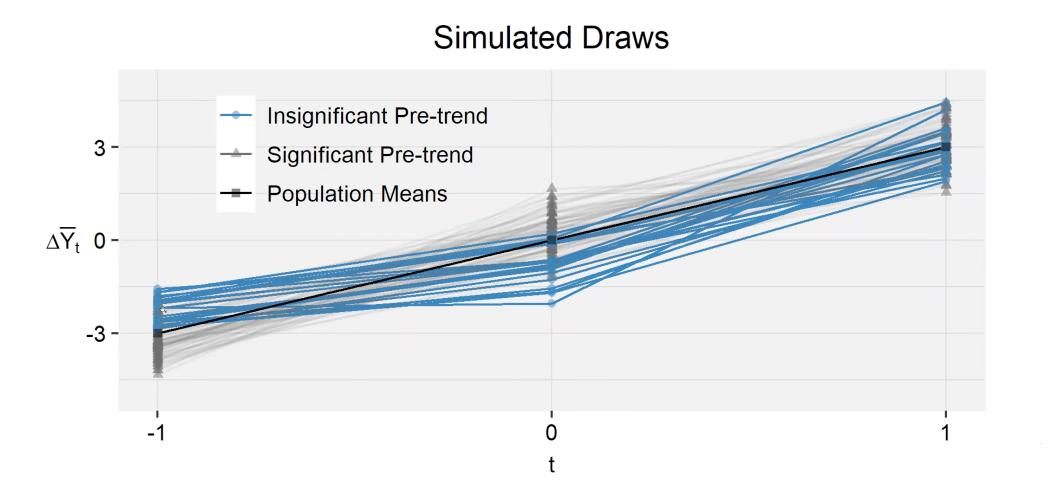
In some of the draws (highlighted in blue), we do not find a significant pre-trend. These are the cases when the outcome at t=-1 has positive error and the outcome at t=0 has negative error. As a result, the post-period effect tends to be particularly large.

In the analysis of past papers, all of them have shown to have insignificant pre-trend (selected sample), it exacerbate the concern that the treatment effect may be overestimated.

It is crucial to acknowledge the limitations of pre-trends testing. Take one step further, what can we do to alleviate these concerns? And if we reject parallel trends in the pre-trends test, does it really mean we cannot learn anything about the treatment effect?

How can we make our DiD analyses more credible?

1. Pre-testing diagnostics

A “low-touch” intervention is to evaluate the likely power or distortions from pre-testing under context-relevant violations of parallel trends. Refer to Pretrends R package.

Pros:

• Very intuitive, easy to visualize
• Helps identify when pre-testing may be least effective
• Requires minimal changes from standard practice

Cons:

• Power will always be <1, so no guarantee of unbiasedness/correct inference
• Need to specify the hypothesized trend, will sometimes be difficult to summarize over many of these
• Still not clear what to do when reject the pre-test

2. HonestDiD

As a more formal tool for robust inference and sensitivity analysis, the HonestDiD approach is more suggestive. It formalizes the intuition above by imposing the restriction that the counterfactual difference in trends cannot be “too different” than the pre-trend. Namely, though we cannot identify the post-period differences in trends (counterfactual), we believe the pre-period difference in trends can be a relatively good proxy for it. This allow us to bound the treatment effect and obtain uniformly valid (“honest”) confidence sets under the imposed restrictions.

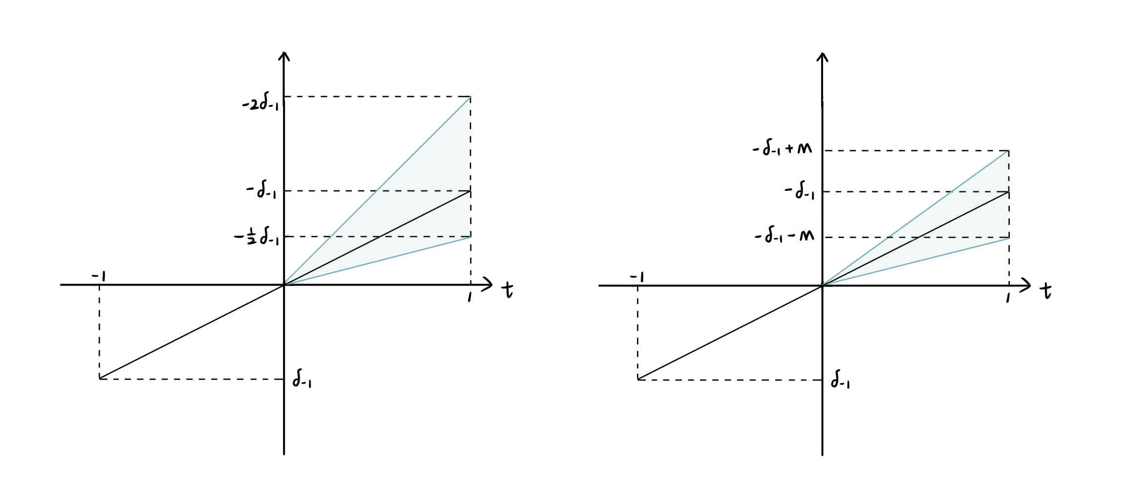
There are two types of restrictions in general. The users should choose the restrictions based on the types of violations of PT you are worried about.

• Bounds on relative magnitudes: $|\delta_{1}|\leq \overline{M}|\delta_{-1}|$ the slope could be difference, but by no more than the magnitude of $\overline{M}$, e.g. industry-specific or macroeconomic shocks that affects treated and controls differently.
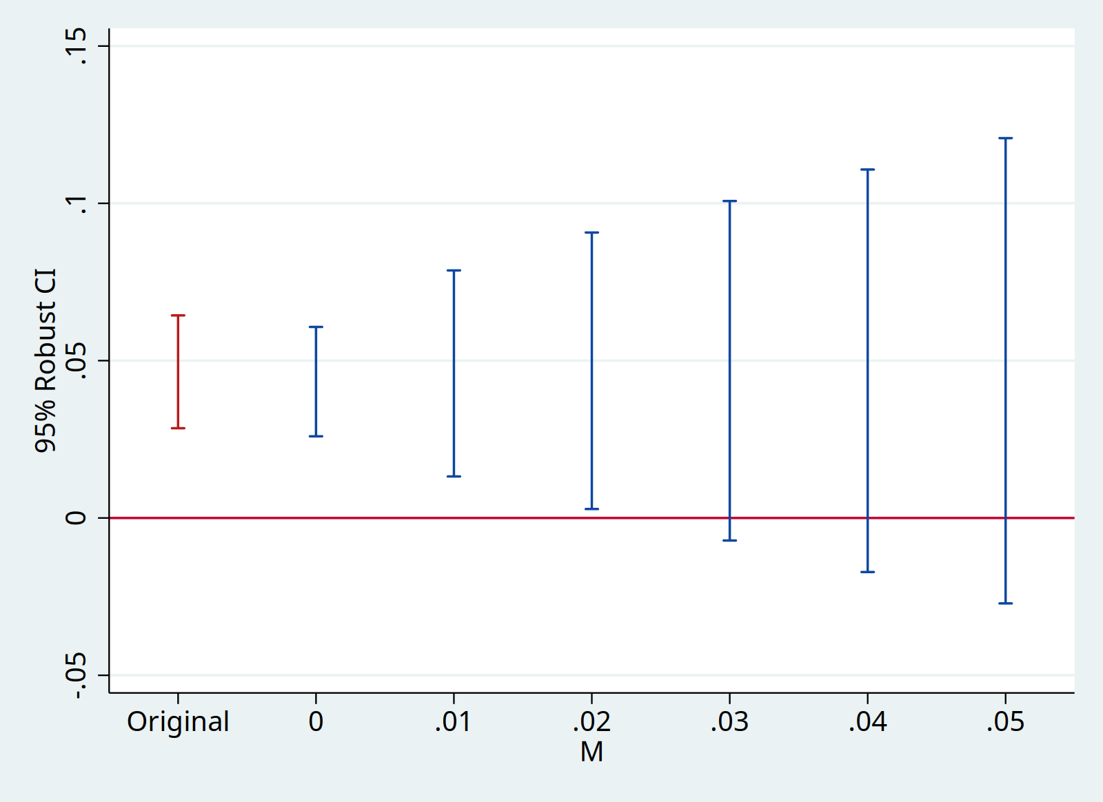
• Smoothness restriction: $\delta_{1}\in [-\delta_{-1}-M,-\delta_{-1}+M]$ bound how far $\delta_{1}$ can deviate from a linear extrapolation of the pre-trend, e.g. smooth long-run trends.

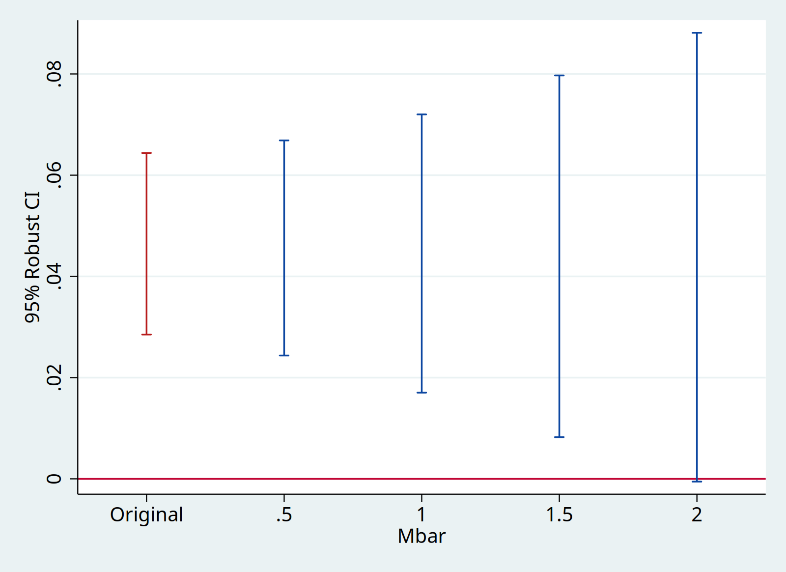
With sensitivity analysis, it allows us to identify the breakdown value. With bounds on relative magnitudes, a breakdown value of $\overline{M}=2$ means the significant result is robust to allowing for violations of parallel trends up to twice as big as the max violation in the pre-treatment period. With smoothness restriction, a breakdown value of $M=0.04$ means the significant result is robust to allowing for the linear change to deviate by 0.04 between consecutive period. The magnitudes need to be interpreted with possible confounds.

For packages and guidelines, refer to

• HonestDiD R package
• HonestDiD Stata package

   // Bounds on relative magnitudes, `mvec(0.5(0.5)2)` tests Mbar equals 0.5, 1, 1.5, 2
   // Average effects, `matrix l_vec = 0.5/0.5` accounts for two post-treatment periods, similar for three or more periods, but make sure the weights add up to 1 
   // Parallel processing, `parallel(4)` number of cores in paratheses
   matrix l_vec = 0.5/0.5
   local plotopts xtitle(Mbar) ytitle(95% Robust CI)
   honestdid, l_vec(l_vec) pre(1/5) post(6/7) mvec(0.5(0.5)2) parallel(4) omit coefplot `plotopts'

   // Smoothness, `mvec(0(0.01)0.05)` tests M equals 0, 0.01, 0.02, 0.03, 0.04, 0.05
   // If `l_vec` is not specified, the default version focused on the effect for the first post-treatment period
   local plotopts xtitle(M) ytitle(95% Robust CI)
   honestdid, pre(1/5) post(6/7) mvec(0(0.01)0.05) delta(sd) omit coefplot `plotopts'

That’s all I have for this post. Thanks for reading, and see you next time!

Reference

• Presentation video by Jonathan Roth
• Rambachan, Ashesh, and Jonathan Roth, 2023, A More Credible Approach to Parallel Trends. Review of Economic Studies, 90 (5): 2555–2591.
• Roth, Jonathan, 2022, Pre-test with Caution: Event-study Estimates After Testing for Parallel Trends. American Economic Review: Insights, 4 (3): 305-322.
• He, Guojun, and Shaoda Wang, 2017, Do College Graduates Serving as Village Officials Help Rural China? American Economic Journal: Applied Economics, 9 (4): 186-215.