
NLP in Finance and Accounting (I): Term Frequency Measure
Published:
In this series of posts, I would like to summarize the current applications of NLP in finance and accounting research, with a focus on how different text-based measurements are constructed. I plan to cover Term Frequency, Text similarity, Sentiment, Readability, BERT.
Before we dive in, I found two survey papers Loughran, Tim, and Bill Mcdonald (2016) and Bae et al. (2022) very helpful for those interested in this strand of literature. I’ve learned and borrowed a lot from them.
In this post, I will share with you the term frequency measures.
Term Frequency Measure
Term-frequency measures are usually used to measure people’s attention to some specific topics. The common way to compute this type of measures is to divide the word count related to a given topic of interest, by the overall length of the document (or transcript). Counting word frequency is straight-forward, while the main issue is usually to construct a word dictionary (library) of interest. For some specific topics like Brexit or Covid-19, it is easy to construct a list of few keywords without too much controversy. But for more wide-ranging topics like political or macroeconomic risk (see papers below), it is almost impossible to do this manually. The most widely-used techniques to address this problem is the pattern-based sequence classification.
The pattern-based sequence classification involves two steps:
- Training: compute the classification strength of a given pattern to each class.
- Select training set with known classification.
- Compute TF-IDF per class for each pattern (e.g. unigrams, bigrams) in the training set, where TF is the number of occurrences of a given pattern in a document scaled by the total number of patterns of the document (measures pattern regularity), IDF is the logarithm of the total number of classes to the number of classes containing the given pattern (measures discriminative power). More details on TF-IDF can be found in my other post on count-based word vectors.
- Classification: classify an unknown document to a particular class.
- Identify matched patterns in the document (those contained in the training set as well).
- Compute the TF-IDF score for each class as the sum of the TF-IDF values for that class of all matched patterns. Higher score indicates that the document is more related to the corresponding class.
- Classify the document to the class with the highest TF-IDF score.
When this technique is applied in finance and accounting, instead of constructing a categorical variable, we often stop at the training step when we select the top N patterns with highest TF-IDF values as our dictionary. Then the topic score of our interest for a given document can be computed as the occurrences of patterns in the dictionary scaled by the total number of patterns in the document. Textbooks and newspaper articles are often chosen as the training set. As for the choice of pattern length, there appears to be large improvements to using bigrams over unigrams in many applications, but even longer patterns appear to work less well.
The pattern-based sequence classification has the advantage that the only subjective choice needed is to choose the training set. This choice is traceable and can be subjected to robustness checks. However, an appropriately labelled training set may not be available, or the vocabulary used in training set could differ from the testing set (e.g. textbooks vs managerial disclosure). Two alternatives can be considered.
- Computer-assisted keyword discovery: it starts with some seed words that unambiguously related to the topics of interest, then the keyword discovery algorithm identifies the remainder of the word list by the co-occurrence with seed words.
- Word embedding: it starts with a set of seed words as well, then uses word embedding to find words that have similar meaning to those seed words. More details related to word embedding can be found in my other posts on Word2Vec and GloVe.
These approaches also limit the number of subjective choices to the initial choice of seed words. Despite this, to empirically prove its validity and robustness, more tests are needed.
- Face validity: show relevant word combinations (unigrams, bigrams) and the text fragments where they occur; distribution of scores across time and across industries; heterogeneity among entities after taking out time and industry fixed effect.
- Audit study based on human reading: hire auditors to verify results using a set of established guidelines. It usually requires great investment to carefully train those auditors and cross-check their results, but helps ensure the accuracy of the measures.
- Convergent validity: it tests the degree of correlation between two measures that theoretically should be associated (e.g. the newly-constructed measures and the existing measures).
- Illustrative case studies: take the example of a single firm to plot its score over time and to explain peaks and troughs in the pattern by significant events.
Related Literature
Below are some examples of how term frequency measures are constructed in the field of finance and accounting. Since the measurement issue is our main interest here, I will skip other parts of those papers (e.g. economic implications), which doesn’t mean they are not important or interesting. You are encouraged to check them out by yourself!
- Hassan et al., 2019: it measures the political risk faced by a given firm-year as the share of their quarterly earnings conference calls that centers on risks associated with politics in general and with specific political topics. To construct a training library of political texts (bigrams), they use an undergraduate textbook on U.S. politics and articles from the political section of U.S. newspapers. Then for a given firm-year observation, the political risk is computed as the number of political bigrams surrounded by a synonym for “risk” or “uncertainty” (within 10 words on either side), divided by the total number of bigrams in the transcript. Each bigram is weighted by its frequency in the political library.

- Flynn & Sastry(2020): it measures the attention toward macroeconomic risks of a given firm-year as the sum of IDF-weighted macroeconomic word frequency. TF-IDF vector for each firm-year communication (10-Q and 10-K) is computed following standard approach. To select the set of macroeconomic words, they calculate TF-IDF for each word appears in 10-Q and 10-K corpus, using TF in each of 3 introductory college-level macroeconomic textbooks and IDF in 10-Q and 10-K filings. Then they rank the top 200 words by this metric in each textbook, and take the intersection among the three books as the final set.

- Andreicovici et al. (2020): it measures the accounting measurement intensity (AMI) of a given firm-year as the number of uniquely-accounting bigrams in its 10-K scaled by the total number of bigrams. They use the FASB pronouncements to construct the accounting training library ($\mathbb{A}$), and a large set of English novels together with BBC news for the non-accounting training library ($\mathbb{N}$). Then the set of uniquely-accounting bigrams is formed as $\mathbb{A}\ \mathbb{N}$. Bigrams that appear in more than 90% of 10-Ks are removed to filter out boilerplate accounting terminology.

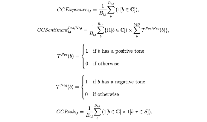
- Sautner et al. (2020): it measures firm-quarter-level climate change exposure as the frequency of climate change bigrams in the conference call transcript scaled by the total number of bigrams. They use a keyword discovery algorithm to produce 4 sets of climate change bigrams, one broadly defined climate change, and three subtopics including opportunity, physical and regulatory. Besides the exposure measures, they also consider two refinements: sentiment measures by considering the presence of positive or negative tone words, risk (uncertainty) measures by considering the presence of risk synonyms in the sentence with climate change keywords.
Li et al. (2020): similar to Sautner et al. (2022), it measures the climate risk of a given firm-year as the share of their quarterly earnings conference calls related to climate risk. The main differences between the two papers are the training dictionary, and the sub-topics chosen under climate change. Li et al. (2020) manually constructs a hybrid dictionary consisting of both unigrams and bigrams related to climate, and separate them into three categories, acute physical climate risk, chronic physical climate risk, and transition risk. To compute the two measures of physical climate risk, they scale the frequency of related keywords (unigrams or bigrams) with at least one risk synonym in their vicinity (±1 sentence) by the length of the transcript. As for transition risk, it is measured based on the occurrences of the keywords in transition risk dictionary only, without requiring them to appear near a risk synonym.
Li et al. (2021): it measures five corporate cultural values for 62,664 firm-year observations over the period 2001–2018. The authors train a word embedding (Word2Vec) model using earnings call transcripts, then construct a culture dictionary based on seed words related to five corporate cultural values: innovation, integrity, quality, respect, and teamwork. The culture scores are TF-IDF weighted.
That’s all I have for this post. If you are also interested in applying NLP techniques to finance research, feel free to check out other pieces.
Stay tuned to this series, see you next time!
Reference
- Andreicovici, Ionela, Laurence van Lent, Valeri Nikolaev, and Ruishen Zhang, 2020, Accounting Measurement Intensity. Working paper.
- Bae, Jihun, Chung Yu Hung, and Laurence van Lent, 2022, Mobilizing Text as Data. Working paper.
- Flynn, Joel P., and Karthik A. Sastry, Attention Cycles. Working paper.
- Hassan, Tarek A, Laurence van Lent, Stephan Hollander, and Ahmed Tahoun, 2019, Firm-Level Political Risk: Measurement and Effects. The Quarterly Journal of Economics 134, 2135–2202.
- Li, Qing, Hongyu Shan, Yuehua Tang, and Vincent Yao, 2020, Corporate Climate Risk: Measurements and Responses. Review of Financial Studies, forthcoming.
- Li, Kai, Feng Mai, Rui Shen, Xinyan Yan, 2021, Measuring Corporate Culture Using Machine Learning. Review of Financial Studies 34, 3265–3315.
- Loughran, Tim, and Bill Mcdonald, 2016, Textual Analysis in Accounting and Finance: A Survey. Journal of Accounting Research 54, 1187–1230.
- Sautner, Zacharias, Laurence van Lent, Grigory Vilkov, and Ruishen Zhang, 2020, Firm-level Climate Change Exposure. Journal of Finance, forthcoming.