
The Divergence of ESG Ratings
Published:
In this post, I will introduce the paper Aggregate Confusion: The Divergence of ESG Ratings by Florian Berg, Julian F Kölbel, and Roberto Rigobon.
To keep a big picture in mind, here are their main findings.
- Though ESG ratings from different rating agencies disagree substantially, it is possible to fit different ratings into a consistent framework.
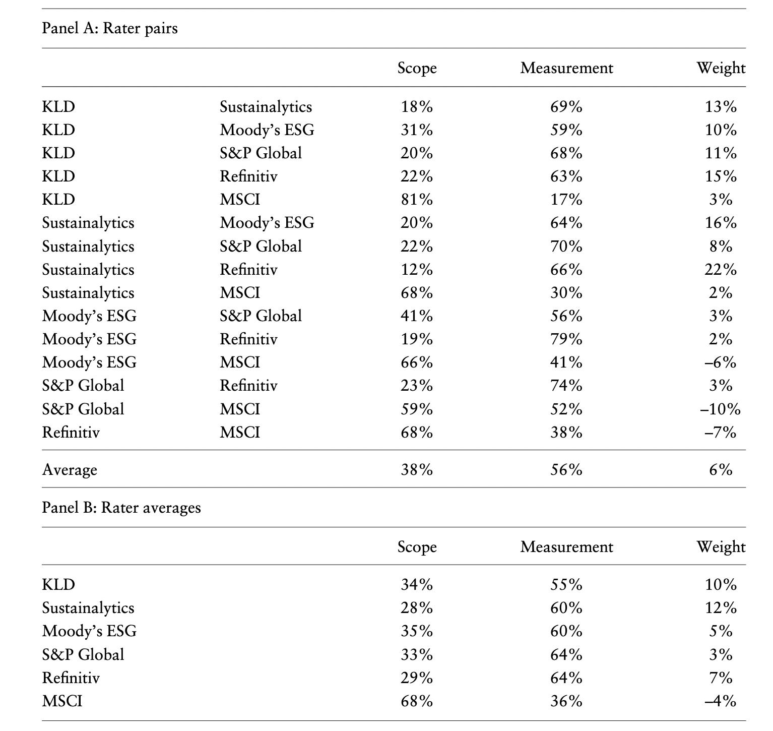
- Measurement divergence is the main driver of rating divergence, contributing 56%, while scope divergence contributes 38%, weight divergence a mere 6%.
- Measurement divergence is in part driven by a “rater effect”, meaning that a firm receiving a high score in one category is more likely to receive high scores in all other categories from that same rater (a rater’s overall view of a firm influences the measurement of specific categories).
Now let’s get into the details.
Motivation
The main motivation of this paper is to examine the drivers of ESG ratings divergence. Below is a visualization of the divergence between the 6 commonly-used ESG ratings from different agencies. Each point represents a pair of normalized ratings, where x-axis is the benchmark rating (Sustainalytics), y-axis is the other ratings (S&P, Moody, KLD, Refinitiv, MSCI in different colors).
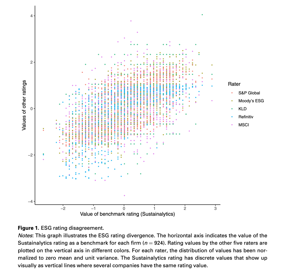
Overall, ESG ratings are positively correlated. However, for any level of the benchmark rating, there is a wide range of values given by other ratings, indicating the substantial divergence. And it will become even more pronounced when other ratings are used as benchmark.
Sources of Divergence
To explain the causes of such divergence, they identify three distinct sources.
Scope divergence
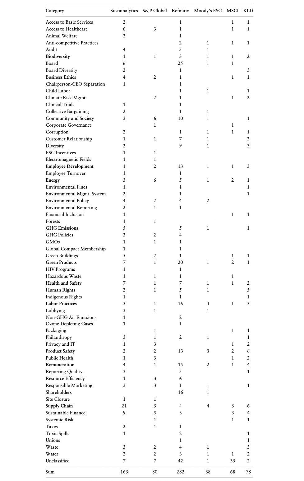
Scope divergence results from rating agencies considering different sets of attributes. As the structures of ESG ratings vary a lot (e.g. different indicators, hierarchies, granularities), the authors develop their own taxonomy as follow to perform a meaningful comparison.
- Create a long list of all available indicators and their detailed descriptions.
- Group indicators that describe the same attribute in the same category.
- Iteratively refine the taxonomy, following two rules
- Each indicator is assigned to only one category.
- A new category is established when at least two indicators from different raters both describe an attribute that is not yet covered by existing categories.
They end up with a taxonomy of 64 categories. Among them, 64 categories are considered by all 6 raters: biodiversity, employee development, energy, green products, health and safety, labor practices, product safety, remuneration, supply chain, water. When comparing two ratings, the difference between categories that are exclusively contained in only one of them can be attributed to scope divergence.
Measurement divergence
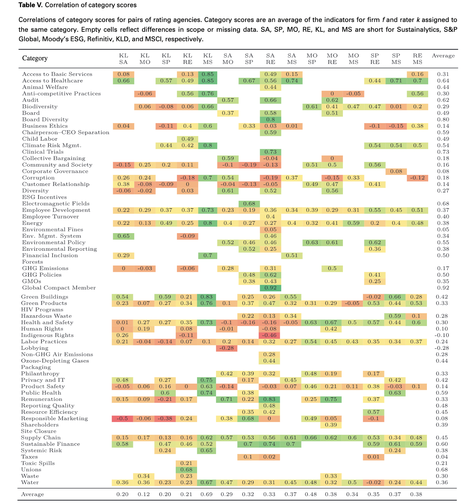
Measurement divergence results from rating agencies measuring the same category with different indicators. To make the assessments of different raters comparable at category-level, category score $C_{fkj}$ is computed as the average of all available indicators of rater $k$ under category $j$ of firm $f$. They compare pairwise correlation of category scores per category and rater pair. Two main insights are
- Correlation levels are heterogeneous. Some of them are even negative, such as lobbying between Sustainalytics and Moody, responsible marketing between KLD and Sustainalytics.
- Correlations tend to be higher in less granular classification. For instance, the average correlation of environmental dimension is 0.53, while only 0.36 and 0.38 for water and energy category respectively. It indicates that divergences compensate for each other to some extent during aggregation.
Weight divergence
Weight divergence results from rating agencies taking different views on the relative importance of attributes. For each rater $k$, they need to estimate the aggregation rule that transform category scores $C_{fkj}$ in to ratings $R_{fk}$. In their main analysis, the authors use a non-negative least squares regression model. Namely, they assume that the aggregation follows a linear function and there is no negative weighs.
\(R_{fk}=\sum_{j\in(1,m)}C_{fkj}\times w_{kj}+\epsilon_{fk}\) where $w_{kj}\geq 0$.
The table below shows their results.
| Rater | Sustainalytics | S&P Global | Refinitiv | Moody’s ESG | MSCI | KLD |
|---|---|---|---|---|---|---|
| $R^2$ | 0.90 | 0.98 | 0.92 | 0.96 | 0.79 | 0.99 |
| Top3 categories | supply chain, environmental management system, green products | employee development, climate risk management, resource efficiency | board, resource efficiency, remuneration | environmental policy, diversity, health and safety | product safety, employee development, corruption | climate risk management, remuneration, product safety |
High $R^2$ values indicate that this linear model could replicate the original ratings quite accurately. The relatively poor performance on MSCI could be explained by industry-specific weights. In the following decomposition, they rely on the fitted ratings computed by category scores $C_{fkj}$ and estimated weighting $\hat{w}_{kj}$.
Decomposition
Now we can perform the arithmetic decomposition to quantify divergence.
For a pair of two raters ${a,b}$, the authors separate their ratings based on common and exclusive categories.
\[\begin{aligned} \hat{R}_{fk}=\hat{R}_{fk,com}+\hat{R}_{fk,ex}=\sum_{j_{com}}C_{fkj_{com}}\times \hat{w}_{kj_{com}}+\sum_{j_{k,ex}}C_{fkj_{k,ex}}\times \hat{w}_{kj_{k,ex}}, k\in \{a,b\} \end{aligned}\]Here, $j_{com}$ represents categories included by both two raters (common categories), while $j_{k,ex}$ represents categories included by rater $k$ but not the other rater (exclusive categories).
Then they decompose the rating differences $\Delta_{fa,b}$ into three components, scope divergence $\Delta_{scope}$, measurement divergence $\Delta_{meas}$ and weight divergence $\Delta_{weights}$.
\[\begin{aligned} \Delta_{fa,b}&=\hat{R}_{fa}-\hat{R}_{fb}=\Delta_{scope}+\Delta_{meas}+\Delta_{weights} \\ \Delta_{scope}&=\hat{R}_{fa,ex}-\hat{R}_{fb,ex}=sum_{j_{a,ex}}C_{faj_{a,ex}}\times \hat{w}_{aj_{a,ex}}-sum_{j_{b,ex}}C_{fbj_{b,ex}}\times \hat{w}_{bj_{b,ex}} \\ \Delta_{meas}&=(C_{faj_{com}}-C_{fbj_{com}})\times \hat{w}^{*} \\ \Delta_{weights}&=C_{faj_{com}}\times (\hat{w}_{aj_{com}}-\hat{w}^{*})-C_{fbj_{com}}\times (\hat{w}_{bj_{com}}-\hat{w}^{*}) \\ \end{aligned}\]where $\hat{w}^{*}$ denotes the identical weights, estimated from pooling regressions using the common categories.
To quantify the contribution of each components to the divergence, they use the variance of $\Delta_{a,b}$ as a measure for divergence (note that all ratings a normalized to a zero mean).
\[\begin{aligned} Var(\Delta_{a,b})=Cov(\Delta_{a,b},\Delta_{a,b})=Cov(\Delta_{a,b},\Delta_{scope})+Cov(\Delta_{a,b},\Delta_{meas})+Cov(\Delta_{a,b},\Delta_{weights}) \end{aligned}\]The results are shown below. On average, measurement divergence is the main driver of rating divergence, contributing 56%, while scope divergence contributes 38%, weight divergence a mere 6%.
The dominance of measurement divergence suggests that it is not merely a matter of varying definitions but a fundamental disagreement about the underlying data. This could be problematic if one accepts the view that ESG ratings should ultimately be based on objective observations that can be ascertained.
The authors perform various robustness checks to ensure that their results are not driven by subjective choices, such as the particular way they built the taxonomy, the functional form to determine rating weights. Detailed results can be found in Online Appendix.
Rater Effect
When further investigating the underlying reasons for measurement divergence, the paper finds the presence of a “rater effect” (also called “halo effect”). Namely, performance in one category influences perceived performance in other categories. This rater effect is evaluated using two procedures
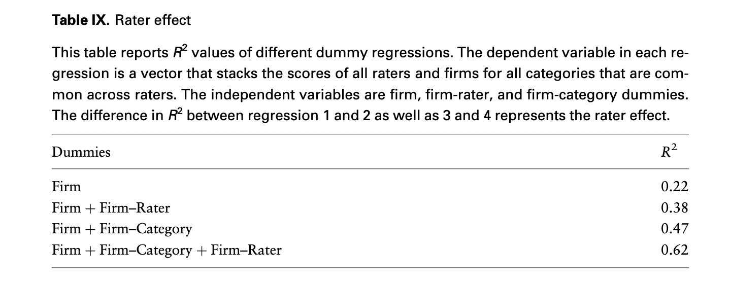
- Rater fixed effects regressions: quantify to what extent the firm-rater fixed effects increase the explanatory power on category scores. From the results below, the firm-rater fixed effects increase the $R^2$ by around 0.15-0.16 (difference between the first and the second specification, or between the third and the fourth). Note that pure rater fixed effects and category fixed effects are dropped due to the normalization at the rating and category scores level.
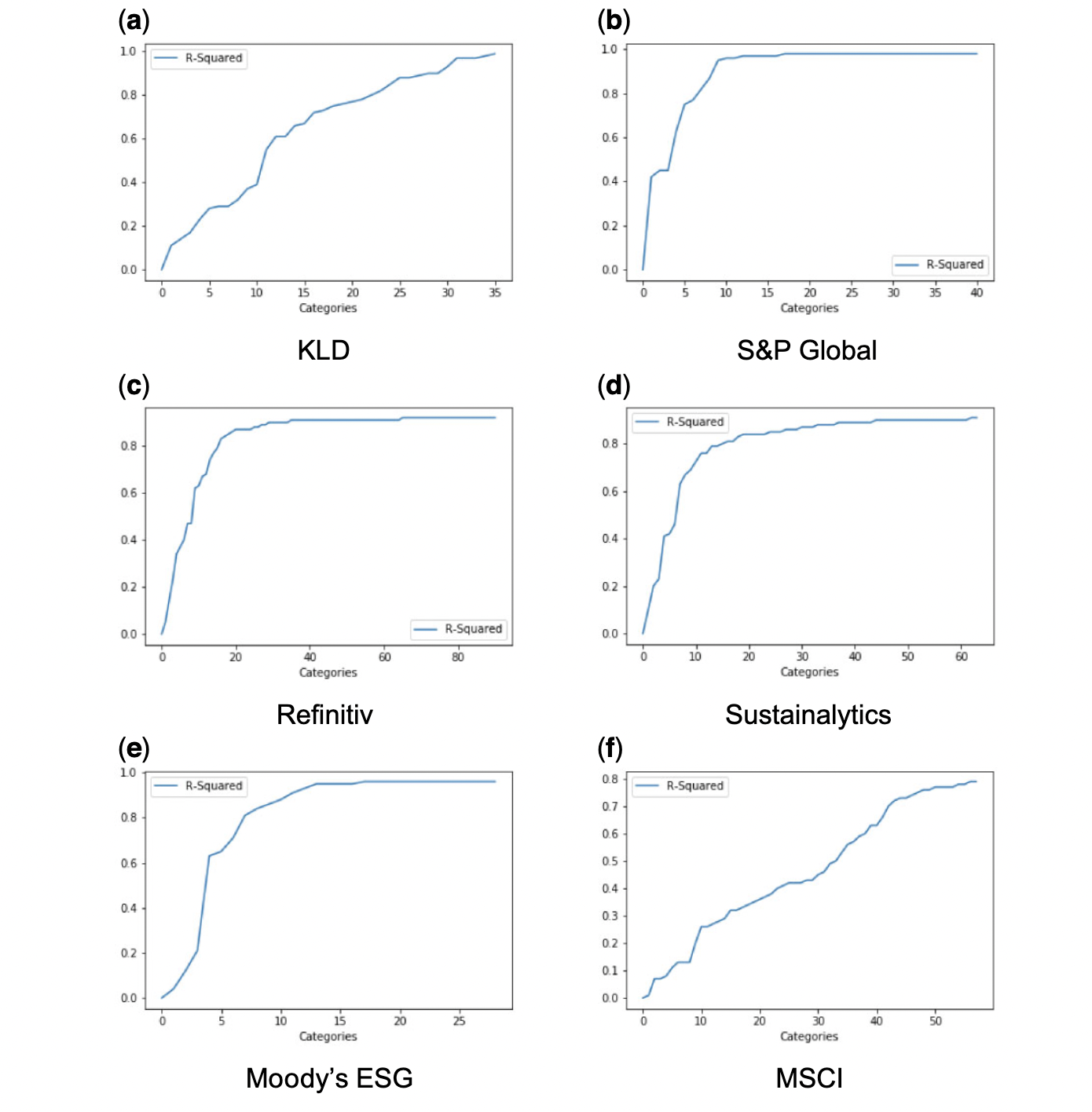
- LASSO approach: estimate the linear aggregation rules with a LASSO regression (penalize non-zero weights). If one can explain the overall rating with less categories, the rater effect will be stronger. From the figure below, the sharp slopes for S&P Global, Refinitiv, Sustainalytics and Moody’s ESG indicate that a few categories already explain most of the ESG rating.
One potential explanation for rater effect is that rating agencies are organized so that analysts specialize in firms rather than indicators. Other potential causes include rater-specific assumptions that systematically affect assessments. For instance, according to S&P Global, it is impossible to get high score if the firm does not answer the corresponding question. The correlation of the probability to answer across indicators could lead to the correlation of category scores.
Contribution and Implication
The contribution of this paper is threefold.
- Among papers on ESG rating divergence, it is the first paper to quantify how much each element (scope, measurement, weight) drives the divergence.
- On the methodological front, it is the first paper to compare several ESG ratings based on the full set of underlying indicators.
- It documents a rater effect, which suggests that measurement divergence is not merely noise but that patterns influence how firms are assessed.
For future studies on ESG, researchers should ideally work with raw data that can be independently verified. If using ESG ratings is inevitable, they provide three suggestions to deal with the rating divergence.
- Include several ratings in the analysis if the intention is to measure consensus ESG performance.
- Use one particular rating to measure a specific company characteristic if it is justified.
- Construct hypotheses around more specific sub-categories of ESG performance to avoid weight and scope divergence.
That’s all about this post. Thanks for reading and hope you find this paper interesting!
Disclaimer: This post is part of my learning note while working on ESG-related projects. Most of the contents are from the original paper, check it out for more details if you are interested.
Reference
- Florian Berg, Julian F Kölbel, and Roberto Rigobon, 2022, Aggregate Confusion: The Divergence of ESG Ratings. Review of Finance, 1-30.