
Word Embedding (II): Word2Vec
Published:
In this article, we will start to discuss prediction-based word vectors. The first model is Word2Vec. We will cover its model structure and implementation.
If you are interested in word embedding, feel free to check out the first post of this series Word Embedding (I): Count-based Word Vectors.
Background
Word2Vec was first published by Mikolov et al. in 2013. As its name implied, Word2Vec maps words to continuous vector representations. In the paper, two new model architectures are proposed, continuous bag-of-words model (CWOB) and continuous skip-gram model. They both use a two-layer neural network to generate word embedding from large corpus like Google news, Wikipedia. The main difference is that they use center word and context word in an inverted way. Skip gram uses center word to predict context words, while CBOW uses context words to predict center word. 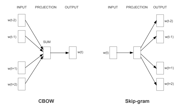
Model performance is evaluated based on word similarities, namely, word occurs in similar context should have similar vectors. In general, skip-gram does a better job in representing less frequent words, while CBOW usually trains faster.
Skip-gram
Skip-gram model predicts the context words o within the window of center word c. It uses neural network with one hidden layer, which is built with a “fake” task. By “fake”, I mean the word embeddings are not the output of the neural network, but the weights of hidden layer and output layer. While the true output is a N×1 vector, where N is the number of unique words in the corpus. Its $i^{th}$ value is the probability of the $i^{th}$ word being the target context word.
Let’s look at the structure of skip-gram model in details. 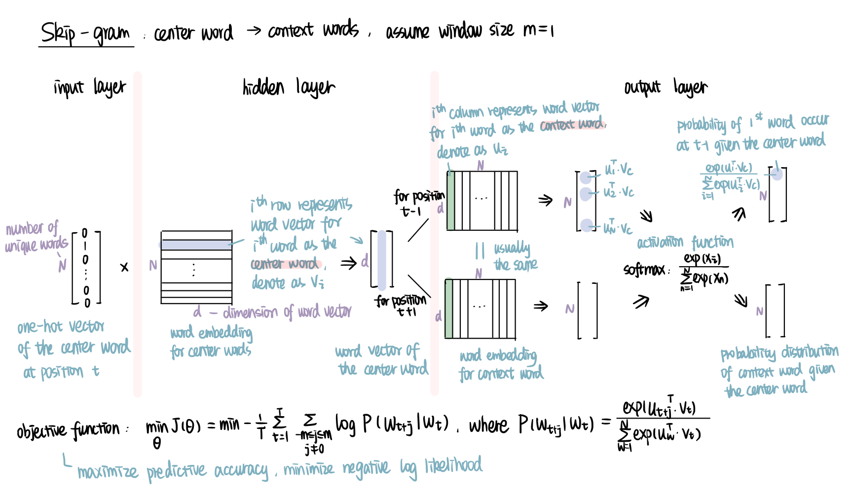
To make this process easier to understand, I will use our small corpus of only 3 sentences and 10 words as an example, and set window size as 1.
corpus = [['the', 'dog', 'is', 'chasing', 'the', 'ball'],
          ['the', 'boy', 'is', 'playing', 'with', 'the', 'ball'],
          ['the', 'girl', 'is', 'crying']]

corpus_words = ['ball','boy','chasing','crying','dog','girl','is','playing','the','with']
The input layer is relative simple. We just need to choose a center word, say 'dog'. Then get its one-hot vector [0 0 0 0 1 0 0 0 0 0], which is a 10×1 vector, and pass it to the hidden layer. If you are not familiar with one-hot vector, check it out here).
In the hidden layer, we mainly do one thing: get the word vector for the center word. To do this, we multiply the transpose of one-hot vector (1×N) with a N×d weight matrix (projection matrix), where d is the dimension of word vector, a hyperparameter that you choose according to your need. For a one-hot vector of the $i^{th}$ word (with the $i^{th}$ element being 1, others being 0), it will give us the $i^{th}$ row of the weight matrix. Word vector is usually in column vector, so we transpose it to get the d×1 word vector, denoted as $v_i$. In our example, we will get the vector for center word 'dog', which is the $5^{th}$ row of the matrix. Note that we do Not have activation in the hidden layer, so we could directly move to the output layer. 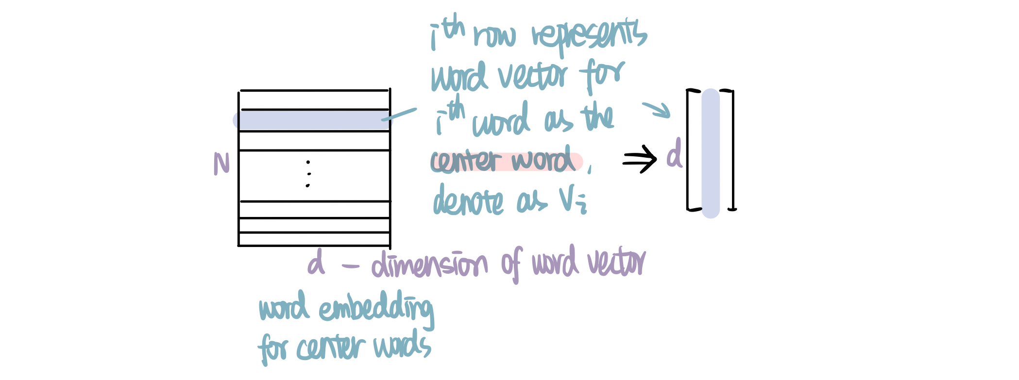
The output layer predicts the probability of a word being the context word given the center word. There are mainly two steps. First, multiply the transpose of $v_i$ with the weight matrix for context word (d×N). Each column of this weight matrix represents the word vector for one context word, denoted as $u_i$. You can think of each dot product $u_i^T\cdot v_c$ as the likelihood of the $i^{th}$ word being in the window of the center word $c$. The greater the value, the higher the likelihood. Second, use softmax activation to normalize and get the probability distribution (N×1). By definition, all values in the output vector add up to 1. Remember our task is to predict the context word surrounding the center word. With 'dog' as the center word, it has two context words around, 'the' and 'is'. So our target output for position t-1 (the one before center word) is [0 0 0 0 0 0 0 0 1 0]. Similarly, [0 0 0 0 0 0 1 0 0 0] for position t+1 (the one after center word). 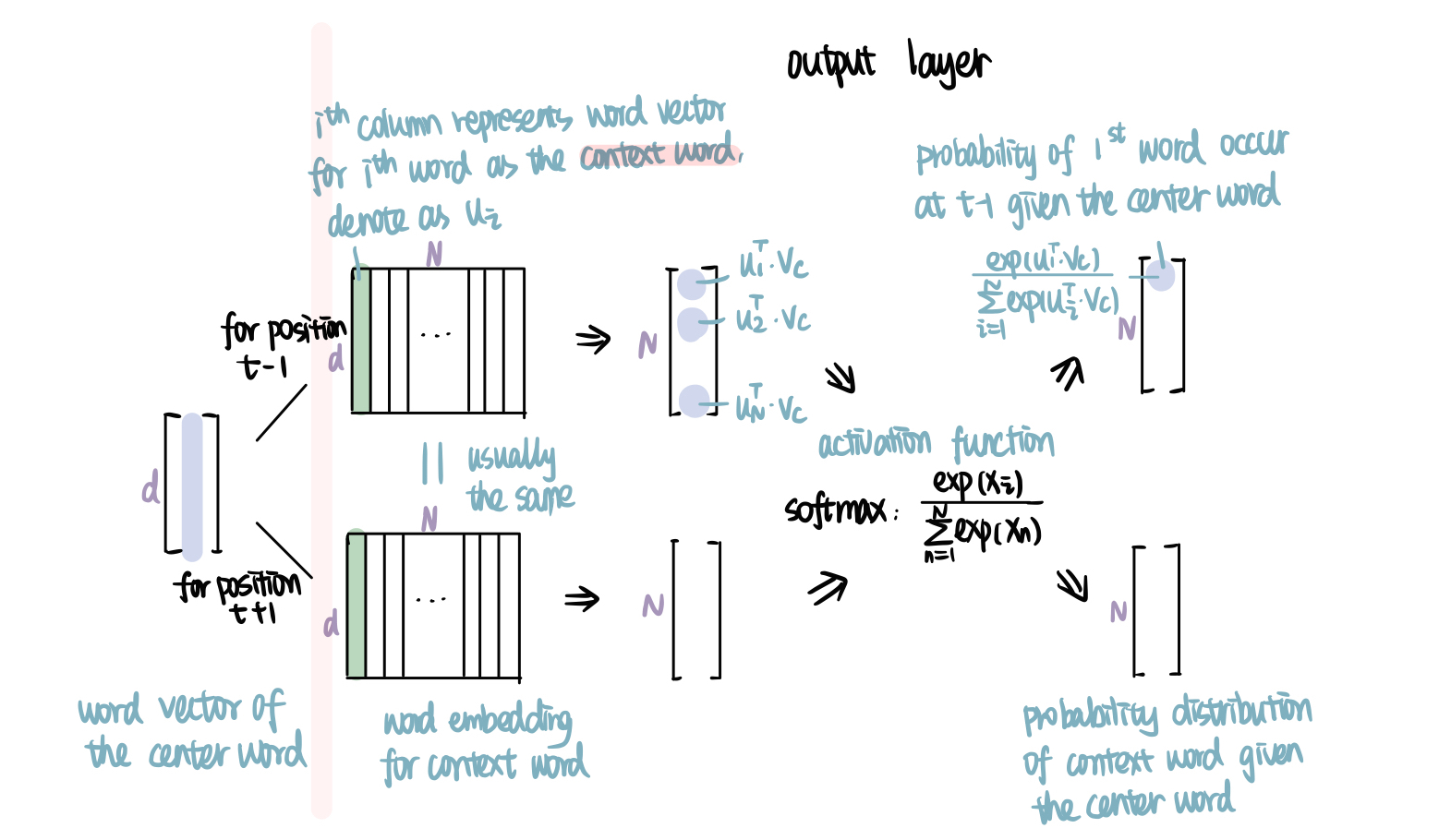
With this model structure in mind, we train the model with pairs of center words and context words from the corpus. In our example, we have 'the' as the center word, ('the','dog'); 'dog' as the center word, ('dog','the'), ('dog','is'); 'is' as the center word, ('is','dog'), ('is','chasing'), ect. If you select a larger window size, you will get more pairs, which usually improves the model performance.
Our objective is to maximize the predictive accuracy, or in other words, minimize the negative log likelihood of the context word given the center word. Write out the loss function \(\min_{\Theta} J(\Theta) = \min -\frac{1}{T}\sum_{t=1}^{T}\sum_{-m\leq j\leq m, j\neq 0} \log P(w_{t+j}|w_t)\), where $P(w_{t+j}|w_t)=\frac{exp(u_{t+j}^T\cdot v_t)}{\sum_{w=1}^{N}exp(u_w^T\cdot v_t)}$. $\Theta$ represents all the model parameters, namely, the two weight matrices in hidden layer and output layer (center word vectors and center word vectors). $t$ represents the position of word, $w_t$ represents the word at position t, $v_t$ represents the center word vector for $w_t$, $u_t$ represents the context word vector for $w_t$.
We use stochastic gradient descent (SGD) to gradually adjust parameters to minimize the loss function. You should heard SGD if you already know some machine learning staffs, if you don’t, a simple explanation would be we adjust $\Theta$ by small step after each training sample in the direction of negative gradient. The step size or learning rate $\alpha$ is another hyperparameter that you need to specify.
After training the model, you get two vectors for each word, $v_t$ and $u_t$. We usually average then to get the word vector for $w_t$.
We can use word similarity to evaluate the model performance. The rationale is that if two words are similar, they should have similar context words, thus, similar output vectors. To make this happen, their weights (word vector) need to be similar. Generally, you could increase the corpus size, vector dimensions or window size to increase the model performance, but that will also increase the training time.
In practice, if we want to get the 300-dimensional vectors for 3 million words and phrases, we need to estimate two weight matrices each with 900 million weights. That’s going to be quite time-consuming for computation. Mikolov et al. address this with the some innovations in their subsequent paper.
- Hierarchical Softmax (HS): it uses a binary Huffman tree to represent the output layer such that it only need to evaluate ln(N) nodes instead of N nodes, more frequent words are assigned with shorter path.
- Negative Sampling (NEG): it matches each training sample with k negative samples, and only updates the weights of the positive word (correct output) and those negative samples, this reduces the weights which need updated in the output layer from N×300 to (k+1)×300, while in the hidden layer, it remains 300 (the word vector for the input center word). k in the range of 5-20 are useful for small training sets, while it can be as small as 2-5 for larger datasets, more frequent words are more likely to be selected as negative samples.
- Subsampling of Frequent Words: more frequent words are less likely to be kept for training, or to put it another way, we are more likely to delete them from the corpus.
CBOW
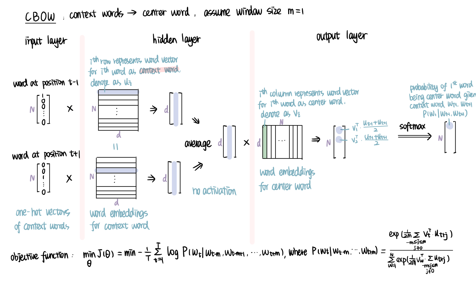
CBOW model predicts the center word based on the context words surrounding it. Same as standard bag-of-words model, the order of words does not influence the projection. But it is continuous in the way that it uses continuous distributed representation of the context.
The structure of CBOW is similar to skip-gram, so I will leave the details for you. The main difference will be it has multiple one-hot vectors of context words as input, and we need to average their vectors before putting into the output layer. The output vector is the probability of each word being the center word given the context words input.
The structure of Word2Vec is similar to NNLM (neural network language model), but they have several differences.
- Objective: Word2Vec aims to get the word embedding (weight matrix), while NNLM aims to predict the next word and the word vectors are by-product.
- Structure: Word2Vec does not use activation function in the hidden layer, while NNLM uses tanh function.
Python implementation
Our final task will be the Python implementation. Gensim makes it a lot more easier for us with ready-to-use models, corpora, and open-source code. Their Documentation and API reference are great places to learn. Check them out if you are interested!
To implement Word2Vec with Gensim, we can use gensim.models.Word2Vec.
import gensim
from gensim.models import Word2Vec

model = gensim.models.Word2Vec(corpus, vector_size = 2, window = 5, min_count = 1)
Below are some commonly used parameters in gensim.models.Word2Vec. You can find out more here.
- vector_size: dimension of word vector, default 100
- window: window size, default 5
- sg: 1 for skip-gram, 0 for CBOW, default 0
- hs: 1 if hierarchical softmax is used, 0 if not, default 0
- negative: number of negative sample chosen (positive integer), 0 if not use negative sampling, default 5
- min_count: ignores all words with total frequency lower than this, default 5
- alpha: initial learning rate, default 0.025
With the model, we can easily get the word embedding for each word, the similarity of two words, the most similar words to the target word. Try them by yourself!
print("word vector of 'boy':",model.wv['boy'])
print("3 most similar words to 'boy':",model.wv.most_similar('boy', topn=3))
print("similarity between 'boy' and 'ball':",model.wv.similarity('boy','ball'))

word vector of 'boy': [-0.24300802 -0.09080088]
3 most similar words to 'boy': [('girl', 0.9593402147293091), ('ball', 0.9566724300384521), ('dog', 0.8807615637779236)]
similarity between 'boy' and 'ball': 0.95667243
Much more can be done with the help of Gensim. For instance, word analogy, we will introduce it in the next post when we talk about GloVe.
That’s all we have for this post. If you find it helpful and want to learn more about word embedding, stay tuned to this series, see you next time!
Reference
- Stanford CS224N | Winter 2021, recordings can be found on Youtube, highly recommended!
- Mikolov et al., 2013, Efficient Estimation of Word Representations in Vector Space
- Mikolov et al., 2013, Distributed Representations of Words and Phrases and their Compositionality
- Genism, models.word2vec – Word2vec embeddings
- Chris McCormick, Word2Vec Tutorial - The Skip-Gram Model
- Chris McCormick, Word2Vec Tutorial Part 2 - Negative Sampling
- Manjeet Singh, Word embedding.